Establishing and Managing the Drug Product Stability Budget

• Eli Lilly and Company

How long can a pharmaceutical product be exposed to temperatures outside the recommended storage conditions? How can product discard be prevented in cases of temperature excursions? How to establish and to manage the allowed time out of storage of a pharmaceutical product? The short answer is: It all depends on the chemical and physical properties of the product, the knowledge about product stability and the presence of temperature exposure data. In this article, the science behind the establishment of a stability budget for products that need to be maintained under controlled temperature conditions will be explored and guidance will be provided to manage the product stability budget in the (bio) pharmaceutical supply chain.

The chemical and physical properties of a drug substance and the drug product formulation determine the product stability and shelf life. During this shelf life pharmaceutical products like vaccines, tablets, crèmes and injectables are exposed to hazards that may impact their quality, efficacy, safety and aesthetics. These hazards may affect the rates of chemical and physical degradation of drug substances and it includes intrinsic factors such as the molecular structure of the drug itself and environmental factors, such as temperature, pH, buffer species, ionic strength, light, oxygen, moisture, additives, and excipients (Yoshioka & Stella, 2002). Temperature is one of the primary hazards that effects drug stability and shelf life. This temperature should be within the allowed and filed conditions established during stability testing programs, which are typically run at the beginning of the product life cycle. In these studies the impact of temperature, moisture (relative humidity), light, shock, vibration, drop, pressure etc. towards the product in its primary marketed package are determined. Here the formation of degradation products and decrease in label claim or potency are measured using stability indicating methods to the end of the product shelf life, which may go to 36 months or longer. During these stability studies, the product is stored under strict controlled conditions in climate chambers at for example +5 ± 3 °C and +25 ±2 °C (ICH 1QA(R2), 2003). At regular intervals samples are drawn from the controlled temperature chambers for testing. From these stability studies, the product shelf life and temperature conditions during manufacturing, packaging, distribution and storage are established (ICH 1QE, 2003)(WHO, 2009). This is not only determined for finished goods, but for drug substances, intermediates and formulated bulk products as well.

The temperature conditions at manufacturing and packaging sites are normally under strict control (GMP regulation) and any temperature deviation with potential impact to a product is investigated. However, as soon as a pharmaceutical product leaves the manufacturing and packaging plant, the level of control is likely to decrease. Especially during transport of these products, many hazards may arise: failure of refrigeration equipment, air flow disruptions, mistakes by employees, extreme weather, exposure to temperature extremes at (air)ports, shipment past the thermal package delivery date, and equipment power interruption are a few examples. If for example strict 2-8 °C storage conditions were to be applied for cold chain products during transportation, then it would be likely that a large portion of the goods would never reach the end customer (the patient) without a temperature excursion. This can happen during loading, in transit and unloading of refrigerated vehicles for example. Establishment of a stability budget that allocates time out of storage (TOS) to distribution activities could help to support temperature excursions within any step in the supply chain and it could eliminate unnecessary discards. Most importantly it can prevent unnecessary drug shortages and maintain the supply of critical medicines to patients.

Most pharmaceutical plants execute the manufacturing and packaging of cold chain products at room temperature (15-25 °C) using the allocated time out of storage (TOS) established by stability studies. The advantages are significant for the company: at room temperature, equipment performs better (less disturbances), label adhesion towards glass vials and syringes is better during secondary packaging, employees can better concentrate (e.g. make less errors while reading procedures), processes and environment are easier to control, and there are fewer temperature excursions compared to the strict 2-8 °C range. A reduction in temperate excursions has a huge advantage as it saves expensive time-consuming investigations, release delay, complexity and discards. However, one disadvantage of allocated TOS is that it may negatively impact the length of the product’s shelf life, which might be important for commercial success of a product. It is therefore a business decision to balance the allocated TOS and shelf life.

Before a pharmaceutical product reaches the patient, it is transported from the pharmaceutical plant via distribution center(s), (pre)wholesaler( s) and point of dispense (e.g. hospital, pharmacy, nursing care facility) using road, air and sometimes ocean as mode of transport. Compared to manufacturing, packaging and storage, the hazards during transportation have the potential for bigger impact due to physical product handling, changing ambient conditions, handovers to other (sub)contracted parties and uncontrolled delays. Thus the allocation of TOS is valuable in order to reduce temperature excursions and discards. Therefore many pharmaceutical companies have set up extended stability studies to determine the minimum and maximum allowed temperatures and time out of storage during transport. For example freeze-thaw cycling and thermal sequential stress studies followed by product shelf life testing (e.g. long term stability testing) might have proven that a product can be exposed for a limited time between -20 and +25 °C, while this product should normally be stored at 2-8°C. The result is a stability budget that allocates TOS to minimum and maximum temperatures during manufacturing, packaging, distribution, storage, atypical events (e.g. failure of refrigerator) and for end users (PDA TR 53, 2011).

Establishment of a Stability Budget

The thermal stability of a drug product should be investigated in order to establish a stability budget for the supply chain. It refers to the quality of a product to resist, under specified conditions, irreversible change in its identity, strength, quality, and purity at various temperatures above and below the labeled claim storage temperature.

Figure 1. The relationship between activation energy (E_a) and enthalpy of formation (ΔH) with and without a catalyst, plotted against the reaction coordinate. The highest energy position (peak position) represents the transition state [D+X]. With the catalyst, the energy required to enter transition state decreases, thereby decreasing the energy required to initiate the reaction.

To establish a stability budget, the rate of the drug degradation should first be determined using long term and accelerated stability studies. This rate depends on several factors including but not limited to the physical and chemical properties of the active pharmaceutical ingredient, formulation, pH, temperature, water and oxygen sensitivity, light sensitivity and primary packaging. Arrhenius argued that for reactants to transform into products, they must first acquire a minimum amount of energy, called the activation energy E_a. Activation energy is equal to the energy barrier that must be exceeded before the degradation occurs (see Figure 1). Arrhenius proposed in 1889 his equation where the activation energy is an independent variable:

The Arrhenius equation is a simple formula for the temperature dependence of reaction rates. This equation gives the dependence of the rate constant k of a chemical reaction at the absolute temperature T (in Kelvin), where A is the pre-exponential factor (or simply the prefactor), E_a is the activation energy (in J mol^-1) and generally 40-130 kJ mol^-1 observed in the degradation of drug substances (Yoshioka & Stella, 2002), and R is the universal gas constant (equal to 8.31446 JK^-1 mol^-1). The Arrhenius equation is valid in the temperature range where both A and E_a in equation (1) can be regarded as constant and it can be used to estimate product shelf life at various temperatures for which stability studies have not been executed (Anderson & Scott, 1991). In addition Arrhenius modeling is most appropriate to estimate k values for temperature ranges for small molecule product degradation that follow zero or first order kinetics (Yoshioka & Stella, 2002). For larger and complex molecules like proteins, k values at various temperatures can be estimated using Arrhenius modeling, but these values should be validated per temperature condition using stability studies.

The units of the pre-exponential factor A are identical to those of the rate constant and will vary depending on the order of the reaction. If the reaction is first order it has the unit s⁻¹, and for that reason it is often called the frequency factor or attempt frequency of the reaction. Most simply, k is the number of collisions that result in a reaction per second, A is the total number of collisions (leading to a reaction or not) per second and e^–Ea/RT is the probability that any given collision will result in a reaction. By either increasing the temperature or decreasing the activation energy (for example through the use of a catalyst) it will result in an increase of the reaction rate.

A first-order reaction depends on the concentration of only one reactant. Other reactants can be present, but each will be zero-order.

Assume that reaction (2) follows first order kinetics and that rate is independent of concentration of reactant [X]. The relationship between the drug concentration [D] after time t for a first order reaction is then

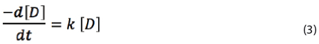
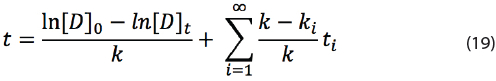
where k is the reaction rate constant at a given temperature T and [D] the concentration of the drug. Rearrangement of equation (3) and integrating from t = 0 to t = t, the following formulas are obtained:

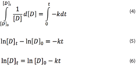
Here [D]₀ is the drug concentration at time t = 0. The rate constant k can be determined using long term and accelerated stability testing.

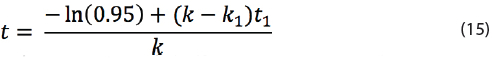
To calculate the shelf life of a drug kept at temperature T with a minimum label claim of 95%, one should replace 0.95[D]₀ = [D]_t in the equation (7):

By eliminating [D]₀ and taking the natural logaritim, one obtains:

Which can be subsequently re-written to

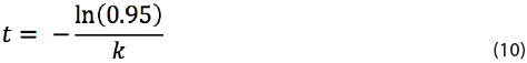
Equation (10) provides the shelf life t of a drug at temperature T with a rate constant k.

Typically the rate constant k is determined from stability studies of a minimum of three batches stored at one temperature and sampled and tested at intervals. Therefore the error in k is affected by the analytical variance and lot-to-lot variance. An appropriate approach to shelf life estimation is to analyze an assay or degradation products by determining the earliest time at which the 95% confidence limit for the mean intersects the proposed acceptance criterion. For example, an assay known to decrease with time, the lower one-sided 95% confidence limit should be compared to the acceptance criterion (ICH 1QE, 2003). Thus t in equation (10) is always larger than the assigned product shelf life in order to accommodate for the analytical variances and lot-to-lot variances. Errors in k are beyond the scope of this article and are not further discussed, but these should be considered when assigning product shelf life.

If a drug during its shelf life is temporarily exposed to a higher temperature, the degradation will be accelerated and thus equation (7) should be multiplied with an additional exponential term e^–k1t1:

Here k₁ is the rate constant at temperature T₁ and t₁ the time at temperature T₁. If t₁ = 0, then equation (11) is equal to equation (7) as e⁰=1. Temporary exposure of the drug to a higher temperature during time t₁ will reduce the shelf life of the drug as the rate constant k₁ is larger than k.

Let’s define t as the maximum shelf life of the drug product. Then the time at storage condition will be shortened from time t to time t-t₁ if exposed to T₁. Thus equation (11) should be rewritten to:

The shelf life time t with a minimum label claim of 95% can be calculated by replacing 0.95[D]₀ = [D]_t in equation (12):

By dividing both sides by [D]₀ and taking the natural logarithm, the following equation is obtained:

Which can be re-arranged into:

Here t is the maximal shelf life of a drug product that is temporarily exposed to high temperature T₁ with rate constant k₁ for time t₁, while the product is normally stored at one temperature T with rate constant k.

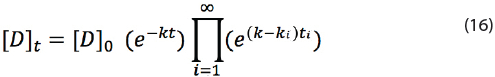
If the product is exposed to multiple different temperatures during its shelf life, then equation (12) can be changed to a general formula:

If i goes from 1 to 2, then the next equation is obtained from equation (16):

The maximum shelf life time t with a minimum label claim of 95% can then be derived to:

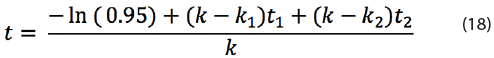
Equation (18) can only be applied to calculate the maximum shelf life if T₁ of k₁ and T₂ of k₂ are larger than T of k. The reason is that T₁ and T₂ are temperature levels that might occur during shelf life. If T₁ or T₂ are below the intended storage conditions, then the shelf life is extended due to lower reaction rate k₁ or k₂. In addition, it doesn’t matter whether the product is exposed at the start or at the end of the product shelf life to the elevated temperatures T₁ and T₂ according to equation (18); the shelf life remains the same.

Equation (18) can be rewritten to a general formula for an infinite number of exposed temperatures above T:

However in practice only 2 to 3 additional conditions are likely to be applied.

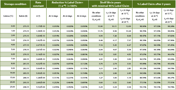
Table 1 shows a list of simulated numbers using the derived equations above. The rate constant k was calculated for each temperature using the Arrhenius equation (1) with A=e^23.1, E_a=104.4 k J mol^-1, and R=8.31446 J K^-1 mol^-1. For each temperature % Label Claim (LC) reduction after 10, 20 and 30 days was calculated using equation (7) assuming a release result of 100.0% and one storage temperature T. The maximum shelf life in years was simulated using equation (18) with minimal 95% Label Claim at end of shelf life. Here the number of years are calculated by dividing t by 31,536,000 seconds (= 365 days x 24 hours x 60 minutes x 60 seconds). The impact of one and two other elevated temperature conditions besides the storage condition during shelf life are listed: 30 days at 25 °C or 20 days at 15 °C plus 10 days at 25 °C. In this example the table shows that if a storage condition of 2-8°C is determined for the drug product, 30 days at 25 °C would not support a shelf life of three years, while 20 days at 15 °C and 10 days at 25 °C in addition to the 2-8 °C storage condition would support a total shelf life of three years (here confidence interval is excluded). The % Label Claim at 3 years was calculated using equation (17) assuming a release result of 100%.

Table 1. Simulated impact of temperature on product shelf life and decrease of label claim.

Using the simulations, the impact of temporary lower and/or elevated temperatures on the drug degradation can be studied. In addition it can provide a proposal to execute real life thermal cycling studies in combination of long term stability testing as more and more regulatory authorities are requesting these kind of real end of shelf life data like Australian TGA (Therapeutic Goods Administration) and ANVISA (Agência Nacional de Vigilância Sanitária (National Health Surveillance Agency Brazil)). For example TGA requires from the applicant for biological medicines with two storage two temperatures (e.g. 1 month at <25 °C and 23 months at 2-8 °C) a study using both temperatures in a worst-case scenario (TGA, 2013). Based on the accelerated stability studies, one can extend the long-term stability study at for example 5 °C by placing the product at a short term elevated temperature condition (e.g. 15 or 25 °C). By applying this approach, filing of TOS for a new product does not have to wait for a new stability study with thermal cycling and long term storage combined.

The principle is to run worst case temperature cycles that represent the temperature exposure of a product during its supply to the end user. The study must start when the product is in the primary container used for testing and ends when the product is at the end of its shelf life. The temperature cycle has to consider the overall TOS and typically temperature conditions:

Figure 2. Simulated stability assay results over time using k = 2.673 x 10^-10 s^-1 (long term at +5 °C in graphs A, C and D) and k₁ = 5.522 x 10^-10 s^-1 (accelerated at +25 °C in graph B (6 months), in graph C at the start (1 month), and in graph D at the end (1 month)), random analytical variance of +/- 0.5%, and lot-to-lot variance of +0.8%, 1.1%, and 0.6% for three lots above release target of 100.0%. Lower bound and upper bound represent the two-sided 95% confidence interval.

• At manufacturing and packaging sites which are normally under strict control under the GMP regulation (manufacturing TOS).
• At distribution sites that may encounter temperature excursions due to unexpected hazards during the shipment of the products from the manufacturing site to the health care provider (distribution TOS).
• At health care providers (e.g. pharmacy, nursery, hospital ) that may encounter temperature excursions during storage and handling of the product (health care provider TOS)
• Here various options can be possible:
• Thermal cycling studies at the start of the product shelf life followed by long term stability testing to the end of shelf life (see simulated assay impact in Figure 2C).
• Long term stability testing and thermal cycling at the end of the (proposed) shelf life (see simulated assay impact in Figure 2D)

The main advantage to establish the stability budget this way is that the data are generated from products exposed during its full shelf life to real temperature excursions and supports regulatory expectations.

Figure 3 provides an example of a stability budget of 720 hours (=30 days) for a pharmaceutical cold chain product with a shelf life of 36 months and 2-8 °C as storage condition.

Figure 3. Example of stability budget of 720 hours (=30 days) for a cold chain product. After mapping of the supply chain, stability budget can be allocated to each step in the supply chain. Process steps marked with a star (*) can have a TOS allocation from +9 to +25 °C (example 1 in Table 1) or +9 to +15 °C (example 2 in Table 1). PDA Technical Report 53 used 720 hours as example as well for a stability budget (PDA TR 53, 2011).

Management of Stability Budget

The stability budget of a pharmaceutical product makes it possible to ensure the product quality, safety and efficacy to the end of the supply chain: the patient. However this can only be achieved if each supply chain partner commits to the following rules:

• A site or supply chain partner is only allowed to use its allocated TOS by the manufacturing site based on an agreement (Quality agreement for example).
• Time and temperature alarm limits of monitors are set to the allocated TOS.
• Temperature is continuously measured and recorded.
• If the allocated TOS is exceeded, remaining TOS at the front of the supply chain can be transferred to site by contacting the supplier in order to save the product.
• It is not allowed to transfer TOS from the end of the supply chain to the front.
• Manufacturing site is the owner of the remaining exposure TOS (if available in the stability budget)
• If a receiving or shipping site has no allocated TOS, the storage conditions must be respected.
• Deviation management system is in place to document and investigate excursions.
• At the point of dispensing, the health care provider or patient may use TOS when indicated in the product leaflet of the manufacturing site.

Each product has its unique physical and chemical properties and thus each product has its own stability profile and temperature sensitivity. A site with 10-20 cold chain products is able to manage each stability budget, but when a site has for example 500 cold chain products in the portfolio, it is almost impossible to manage all individual stability budgets of those products. In such situation, categorization of products must be applied to manage the stability budgets and to simplify the operations by comparing the stability budgets of various products. Table 2 provides an example list of categories for products stored at 2-8 °C.

Table 2: Example stability budget categorizations of products.

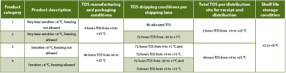
By applying the stability budget categorization approach, the number of temperature monitor types can be significantly reduced for shipments and it simplifies the operations within the warehouses.

Most warehouses have premises at room temperature. Thus if a cold chain product needs to be shipped it goes from the cold store via the premise to the refrigerated truck for example. During this transit the product will be exposed to room temperatures and thus TOS should be available. Typically one hour TOS from +9 to +25 °C should be sufficient to load a cold chain product into a refrigerated truck and one hour TOS from +9 to +25 °C to provide the truck the time to equilibrate within the +2 to +8 °C range. But also at the receiving site, TOS should be available in order to unload the product from the truck. If no TOS is available protective measures like refrigerated premise or thermal covers can be applied in order to comply to the storage conditions. Thus ideally each site should have a minimum of 2-4 hours TOS from +9 to +25 °C per cold chain product with a storage condition of +2 to +8 °C to cover inbound and outbound excursions and to cover in transit temperature excursions due to door openings of refrigerated trucks or vans.

Conclusion

The stability budget concept is an effective management tool to allocate time out of storage to each supply chain partner for the manufacturing, packaging, storage and distribution of (bio)pharmaceutical products. It ensures that the products maintain the intended quality, safety, efficacy and esthetics to the end of the supply chain and shelf life if each site commits to the stability budget rules and allocated TOS. The stability budget concept can be applied for all type of products including products with storage conditions at < -20 °C, 2-8 °C and 15-25 °C.

The establishment of stability budgets for (bio)pharmaceutical products provide benefits for the supply chain as it simplifies operations by reducing the expensive time-consuming investigations of temperature excursions. Thus it accelerates the release and availability of a shipped product to the next stage in the supply chain. Finally, stability budgets will help to reduce the cost of unnecessary discard and drug shortage and thus it can save and extend the life of the products to be used by the patients.

Acknowledgement

The authors would like to thank Arjen Loebis (MSD), Sally Wong (Merck & Co.), Robert H. Seevers, PhD (Eli Lilly and Company) and Fabian De Paoli (GSK) for their review and comments while preparing the manuscript of this article.

References

1. Anderson, G., & Scott, M. (1991). Determination of product shelf life and activation energy for five drug of abuse. Clin. Chem. 37/3, 398-402.
2. ICH 1QA(R2). (2003). Stability testing of new drug substances and products.
3. ICH 1QE. (2003). Evaluation for stability data.
4. PDA TR 53. (2011). Guidance for industry: Stability testing to support distribution of new drug products.
5. TGA. (2013). Guidance 14: Stability testing for prescription medicines (Previously ARGPM 14: Stability testing), 31 July 2013 (https://www.tga.gov.au/book/export/html/4157).
6. WHO. (2009). Stability testing of active pharmaceutical ingredients and finished pharmaceutical products. WHO Technical Report Series, No. 953, 87-130.
7. Yoshioka, S., & Stella, V. J. (2002). Stability of Drugs and dosage forms.

Erik J. van Asselt, PhD ([email protected]) is Improvement Engineer at MSD in The Netherlands and the Leader of the Parenteral Drug Association (PDA) Pharmaceutical Cold Chain Interest Group (PCCIG), EU Branch.

Rafik H. Bishara, PhD ([email protected]) is a Technical Advisor and the Leader of the Parenteral Drug Association (PDA) Pharmaceutical Cold Chain Interest Group (PCCIG), US Branch.